Nonlinear Averaging
The principle of nonlinear averaging is simply that the average of a function is not the same as the function evaluated at its average.
The principle is mathematically formulated by Jensen's Inequality (equation below), but is best understood with a biological example. 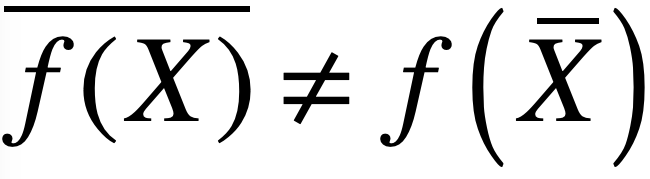
Say you do an experiment with predators and prey. You set the experiment up to find how many prey are eaten with different number of predators. You set up 5 arenas, with 0, 1, 2, 3, 4, and 5 predators. The results you get (in a perfect world) look like the blue points in the figure at the right.
The blue curve is an exponential function (call it f) that fit to this data and describes how likely any prey is to be consumed given some number of predators around. |
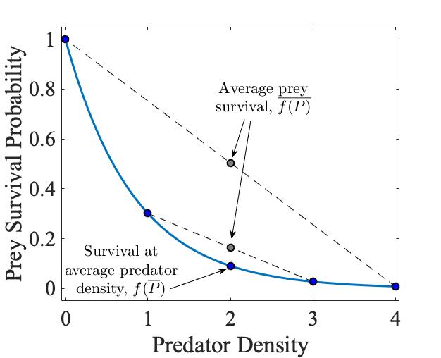
Now, one might wonder how many prey would survive if the landscape had the average predator density of 2, f(P =2)? That is shown in the figure. But what if there were two patches, with different predator numbers, but the same average? Depending on the variability, the average survival rate is much higher in these instances because areas with few predators lead to much higher survival. The average survival in two cases is given by the gray points.
Such nonlinear averaging is relevant to quantitative analysis of many biological questions. It relies on nonlinearities in the biology and variability of components. Both are ubiquitous in ecology and evolutionary biology. |
